When Edge Meets Learning: Adaptive Control for Resource-Constrained Distributed Machine Learning
2018年IEEE INFOCOM
人与人之间的差距不能一概而论…
0x00 Abstract
We analyze the convergence rate of distributed gradient descent from a theoretical point of view, based on which we propose a control algorithm that determines the best trade-off between local update and global parameter aggregation to minimize the loss function under a given resource budget. The performance of the proposed algorithm is evaluated via extensive experiments with real datasets, both on a networked prototype system and in a larger-scale simulated environment.
Key Words: Convergence Rate,Federated Learning, Resource Budget
0x01 INTRODUCTION
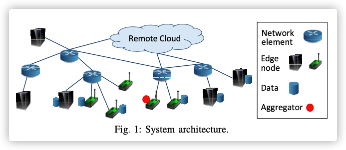
In this paper, we address the problem of how to efficiently utilize the limited computation and communication resources at the edge for the optimal learning performance.We consider a typical edge computing architecture where edge nodes are interconnected with the remote cloud via network elements, such as gateways and routers.
The frequency of global aggregation is configurable; one can aggregate at an interval of one or multiple local updates. Each local update consumes computation resource of the edge node, and each global aggregation consumes communication resource of the network. The amount of con- sumed resources may vary over time, and there is a complex relationship among the frequency of global aggregation, the model training accuracy, and resource consumption.
Main contributions:
- We analyze the convergence rate of gradient-descent based distributed learning from a theoretical perspective, and obtain a novel convergence bound that incorporates non-i.i.d. data distributions among nodes and an arbitrary number of local updates between two global aggregations.
- Using the above theoretical result, we propose a control algorithm that learns the data distribution, system dynamics, and model characteristics, based on which it dynamically adapts the frequency of global aggregation in real time to minimize the learning loss under a fixed resource budget.
- Experiments
0x02 RELATED WORK
0x03 PRELIMINARIES AND DEFINITIONS
A.Loss Function
下标表示节点信息;没有下标的表示全局信息。
B.The Learning Problem
找到权重的最优值,没有解析解,只能用梯度下降。
C.Distributed Gradient Descent
由联邦学习的特征可知,当本地一定轮数后,就会进行全局模型聚合。所以对节点上某次迭代来说,最后的模型要么就是单纯的本地训练模型,要么就是全局聚合的模型。
用 表示第迭代获得模型参数:
其中
是利用梯度下降计算:
是带权聚合:

总共会执行次节点本地计算,每次聚合一次,所以整个训练过程会聚合(为了方便,只考虑其为整数),
The rationale behind Algorithm 1 is that when , i.e., when we perform global aggregation after every local update step, the distributed gradient descent (ignoring communication aspects) is equivalent to the centralized gradient descent, where the latter assumes that all data samples are available at a centralized location and the global loss function and its gradient can be observed directly. This is due to the linearity of the gradient operator.
0x04 PROBLEM FORMULATION
The notion of “resources” here is generic and can include time, energy, monetary cost etc. related to both computation and communication.
Therefore, a natural question is how to make efficient use of a given amount of resources to minimize the loss function of model training. For the distributed gradient-descent based learning approach presented above, the question narrows down to determining the optimal values of and , so that is minimized subject to a given resource constraint for this learning task.
Formally, we define that each step of local update at all participating nodes consumes units of resource, and each step of global aggregation consumes units of resource,where and $ b≥0$ are both real numbers.
For given and , the total amount of consumed resource is then . Let denote the total resource budget.
Further, the resource consumptions and can be time-varying in practice which makes the problem
even more challenging than (6) alone.
目标问题:
0x05 CONVERGENCE ANALYSIS
A.Definitions
为了找出的上界,先引入一写定义:
- ,表示整个训练过程有个间隔(interval)
- ,表示一个间隔
- :在区间的辅助参数向量
表示中心化梯度下降的,对集中式的梯度下降是研究比较多的,也是分布式梯度下降的性能天花板。
此时的损失函数能够访问任何样本(解释了下图,为何下降快)
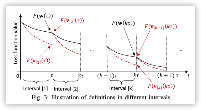
观察上图:
-
在的整数倍(分割线处),就会进行全局聚合,即
-
在间隔界限上,
这个图可以理解成为上帝视角,所以才能观测出连续的全局损失变化。
为了获得算法1的收敛界限需要分两步走:
- 获得每个间距的与的差距
- 将这个差距和的收敛速度相结合,获得的收敛速度
是集中式的梯度下降,收敛速度较容易获得,再加之某个时间段的积累差距,以此来估计的速度
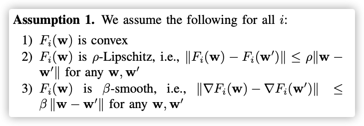
Lemma 1: is convex, -Lipschitz, and -smooth.
: This is straightforward from Assumption 1, the definition of F(w), and triangle inequality.
Definition 1:(Gradient Divergence)
For any and , we define as an upper bound of ,i.e.,
We also define
B.Main Results
Theorem 1.
For any interval and , we have
where
for any . Furthermore, as $F (\cdot) $ is -Lipschitz, we have .
:数学归纳法,有空再细看
Theorem 2.
The convergence upper bound of Algorithm 1 after iterations is given by
when the following conditions are satisfied:
- for all and for which is defined
- Where and
:没看。。。
0x06 CONTROL ALGORITHM
A.Approximate Solution to (6)
根据公式(6)和定理2,目标问题如下:
当和设置的较小,能满足定理2的要求的时候,公式(12)可以转换成如下:
The optimal solution to (13) always satisfies condition 2 in Theorem 2, because (in which case ) yields the objective function to be positive and thus satisfying the condition.
公式(13)除以,则目标函数如下,其中定义:
现在我们的目标就是寻找最优的:
然后就能获得最优的.
Proposition 1.
When , is a strictly concave function for .
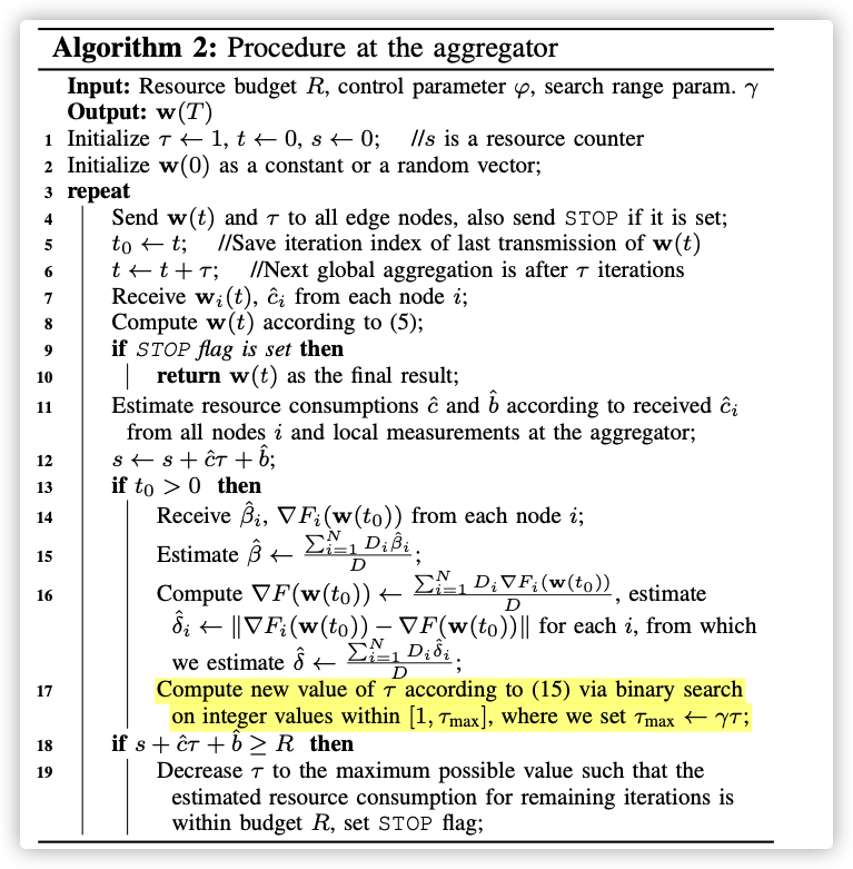
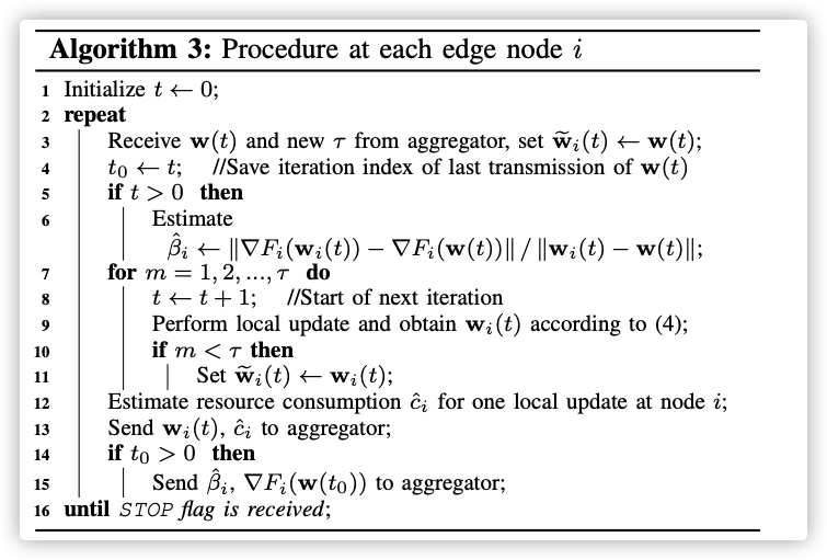
B.Dynamic Control Algorithm
其中超参数确定后
参考
- 伯努利不等式
- 凸优化
 wechat