Heterogeneous Federated Learning

下载链接

0x00 Abstract

• 为了解决数据分散的问题，提出了一种新的联邦学习框架，协作模型之间建立牢固的结构信息对齐方式。

• 设计一种特征定向提取的方法($\varPsi-Net$)，该方法能确保在不同的网络中都有明确的特征信息。

KEY WORDS: Permutation invariance,FedAvg,Convergence

0x01 Introduction

• FedAvg算法在高度Non-IID的情况下，性能损失会很严重。

• 不同节点的初始模型是相同的，但是在不同的本地数据训练的情况下，导致了参数的不同，这就是基于坐标平均的缺点。

• 已经有学者研究"Permutation invariance"等方式，但任然存在参数不精确匹配、额外计算、扩展性差等局限性。

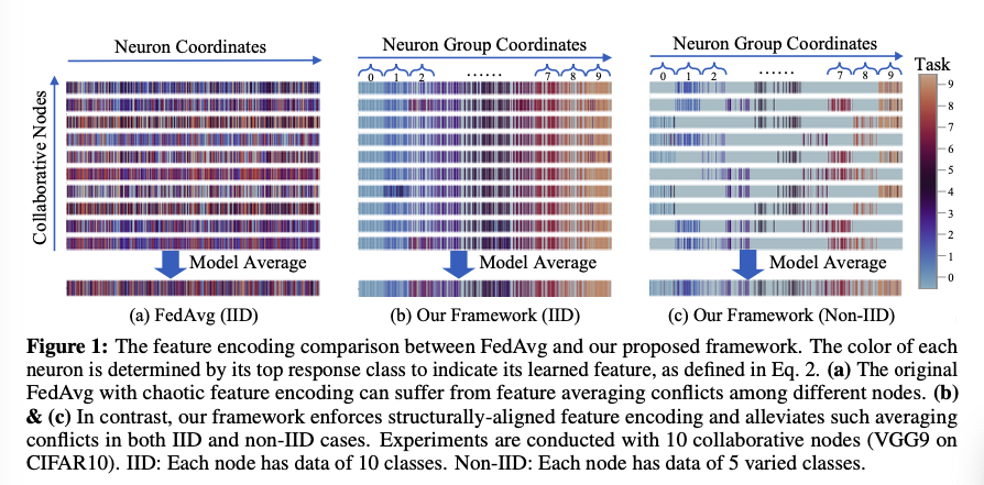
• 为了解决上述限制问题，我们提出了自己基于结构和信息对齐的FL架构。下图展示对比FedAvg的优点：

  

0x02 Background and Motivation

Neural Network Permutation Invariance

$$F(X) = (\omega_0\Pi_0)\Pi_0^{T}X =...=(\omega_i\Pi_i)\Pi_i^{T}X=...=(\omega_N\Pi_N)\Pi_N^{T}X$$

$\omega_i$是权重矩阵，$\Pi_i$是置换矩阵

协作节点的全局函数是相同的，但是置换矩阵的不同导致匹配的参数不同($\omega_i\Pi_i≠\omega_j\Pi_j$)，使得性能下降。

Matched Averaging with Permutation Adjustment

为了实现模型对齐，以前的工作是在全局平均周期之前，将近似参数与置换进行匹配。过程如下：

• 根据不同节点评估特定参数特征获取的标量值，定义近似参数。
• 寻找调整矩阵$\Pi^{trans},s.t. \omega_i\Pi_i\Pi^{trans}≈\omega_j\Pi_j$
• 参考Wasserstein Barycenter problem

Limitations of the State of the Art

• 不准确的参数匹配
• 异质适应性
• 计算开支
• 数据隐私

Design Motivation:Feature-Level Alignment

• 进一步解释神经网络中编码特征信息，将参数相似性评估提升到特征相似。
• 本文设计了一种特征导向模型规范的方法，确保特定模型结构中的明确特征分配。

结合上述两点，本文工作首先解释编码特征信息：采用类别响应偏好(class response preference)的方式学习特征。

Example:

在分类任务的全连接层，”偏好“可以设置为神经元激活响应$A(x_c),x \in Class\ C$;也可以是预测可信度($Z_c$)对其偏导:$\partial Z_c/\partial A(x_c)$。

结合上述两个因素，用类别偏好向量(class preference vector)表示神经元学习的特征：

$$P=[p_1,...,p_c,...,p_C],Where\ p_c=\sum\limits_{b}^{B}A(x_c,b)*\frac{\partial Z_c}{\partial A(x_c,b)}$$

注：$B$表示聚合批次大小。

OUR WORK:Feature-Allocated Model Regulation and Collaboration

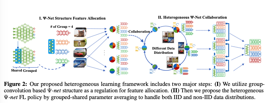
本文提出的网络由分享层(shared)和分组层(grouped)构成，用于分享全类的基础特征和高级结构里的分类特征(class-specific features)。

优点：

• 可以用于不同的训练阶段
• 可以为不同的FL场景做优化
• 可以适用于极度异质情况(部分类别不能从部分节点学习)

0x03 $\varPsi-Net$ Structure for Feature Allocation

1. Feature Allocation Definition

在模型元结构集合$S$与任务集合$T$之间采用结构-特征映射关系$M$：

$$M = \{s_i^t:t\ or\ <t_0,...,t_n>\},s.t. \forall i≠j,M(s_i)\cap M(s_j)=\empty$$

where $s_i^t$ indicates one meta-structure (e.g., one set of neurons in the neural network) mapped to one (or one set of) task feature $t$, and $M(s^{t_1}) ∩ M(s^{t_2}) = ∅$ enforces that any individual task feature can be assigned to only one meta-architecture.

本文假说应用于密集的卷积层。

• $\varPsi-net$利用了分组卷积和线性层构建元结构集合$S$.

• 通过将$logit\ t$分配给结构组$s_i$,完成将任务$t$的特征分配给结构$s$的假设,$s_i→s_i^t$.

• 通过这种方式，将$s_t^t$作为任务t的特征”anchor“，这就保证了下面条件的成立：

  $$\Omega_t←s_i^t≈...≈s_j^t≈...≈s_N^t,\forall i,j\in N$$

  Meanwhile, even though different nodes can have varied structure orders, their local structure $s_i^t$ can still be explictly mapped with the $Ω_t$, which is the t-th meta-structure in the global model structure $Ω$.

有了这种特征对齐属性，就可以加强结构特征对齐，实现异质模型的协作。

2. $\varPsi-Net$ Structure Implementation

组成部分：Non-grouped shared layers (lower convolutional layers) and grouped layers (higher convolutional and fully-connected layers).

宗旨：每个分组学习指定的任务特征。

Shared Layers.

目的：浅层学习能获得大多数任务的基础特性，很少的特征差异。

对基础层分组能防止接收其他组的梯度传播，从而导致次优的学习性能。（因此浅层只保留共享，而不分组。？？？）

选择合适的浅层数目，评估该层的特征总方差：

$$TV_l=\sum\limits_{i}^L \frac{1}{L}||P_{l,i}-E(P_{l,i})||_2,where\ P_{l,i}=[{p_{l,1},..,p_{l,N}}]/\sum\limits_{j}^Np_{l,j}$$

Group Convolutional Layers.

在较深的卷积层，编码后的分类特征会有很大的差异，这在聚合的时候很容易产生性能损失。

采取分组卷积，能够有效避免性能损失。

在复杂的数据集上，分组数与训练任务数并不是一对一的，允许一对多。

Group Fully-Connected Layers.

卷积层的神经元与每个class logits相连接，就无法调节分组卷积获得的相关特征。

将FC分组，分成与分组卷积层具有相同编号的线性层。

一个线性层只与一个卷积组相关联，不会导致反向传播的交叉。

Group Normalization Layers.

Batch Normalization Layers能够影响FL模型的效能，因为不同节点使用的数据差异。

在分组卷积层后添加GN层、是为了提高模型收敛速度。

0x04 $\varPsi-Net$ Collaboration for Heterogeneous Federated Learning

展示一个具体FL协作框架

Global&Local Model Initialization.

全局模型和本地模型的初始化过程是不同的。

**Globel Model:**给定多分类的学习任务和目标网络架构后，上面提到的正则化方法会确定shared layers和grouped layers的层数。

Local Model：

• 在IID和普通non-IID的情况下，本地模型初始化和全局模型是相同的。
• 在极端non-IID情况下，采用不同的模型进行初始化。（对模型的分组结构进行剪枝）
  • “one-to-one”:本地没有任务数据直接被剪枝
  • “one-to-many”:只有本地数据都满足该组的任务，该组才会被剪枝。

Local Model Training.

正常进行本地模型训练。

• 与SOTA相比，结构信息对齐可以持续进行，少了参数分享、评估、再对齐等大量计算开销。
• 非对称任务节点对模型剪枝，减少了计算成本。

Aligned Model Averaging.

聚合操作每$e\ epoches$进行一次。

Shared layers.

因为是提取基础特征，所以特征差异较小，所以可以直接聚合。

$$\Omega_{shared}=Avg(\omega_{shared}^i),\ i \in \{1,...,N\}$$

Grouped layers.

只有相对应的类才会进行聚合,例如对class c的分组进行聚合：

$$\Omega_c = Avg(\omega_c^{I_c}),\ I_c = \{i,s.t. c\in M(i)\}$$

在非极端non-IID(未剪枝的情况下)，$I_c$包含全部的节点。

Normalization layers.

分为 Batch Normalization Layer和 Group Normalization Layer。

For batch normalization in shared layers, we average the “shift” and“ scale” parameters, as well as the the “running_mean” and “running_variance” statistics for each layer.

For group normalization in the grouped layers, only the “shift” and “scale” parameters are averaged within matched groups, as the other two are subject to the batch change.

Heterogeneous Model Collection.

将极端Non-IID情况考虑进去的话，全局模型表示如下：

$$\Omega^{Globel} = \{\Omega_{shared},\Omega_1,...,\Omega_C\}$$

0x05 Experiment

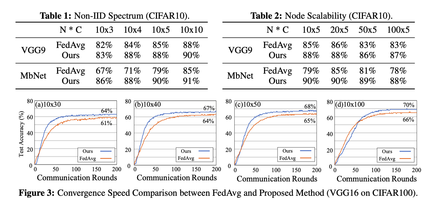
数据集：CIFAR10、CIFAR100

网络架构：VGG9、VGG16、MobileNetv1。（用于证明本文结构调整方法的一般性）

Non/IID：non-IID拥有数据集的部分类。

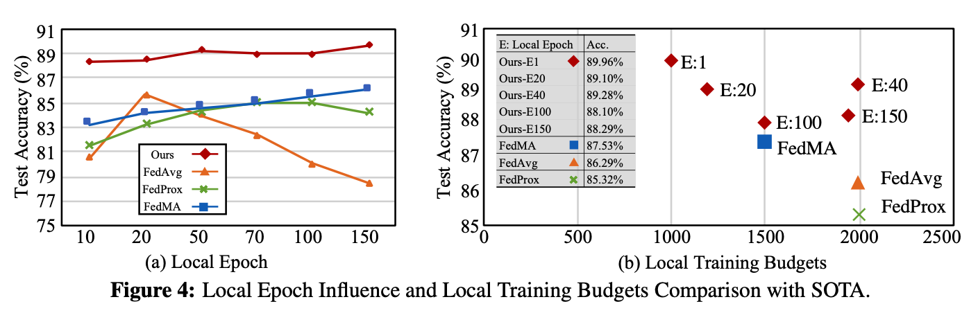
SOTA：FedMA、FedProx（作为对照组）

1.Convergence Perfomance Improvement Evaluation

2.Performance Comparison with SOTA (FedProx & FedMA)

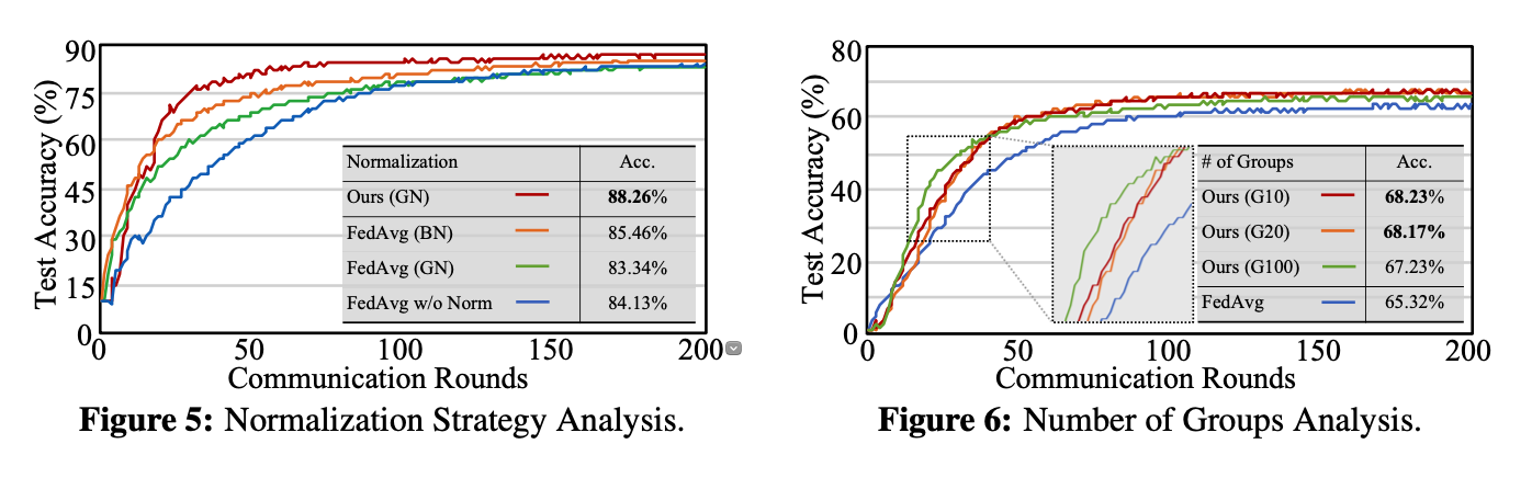
3.Ablation Study of Design Components

We study the performance influence of three design strategies in our framework, including the normalization layer influence, grouping number selection, as well as the sharing layer depth selection.

Normalization Strategy Analysis.

For normalization strategy analysis, we compare our work and FedAvg under the data distribution of (VGG9, CIFAR10, 10x4 non-IID). The results are shown in Fig. 5. The baseline FedAvg without normalization achieves 84.13% accuracy. FedAvg+BN helps improve the accuracy to 85.46%, while FedAvg+GN hurts the model performance, degrading the accuracy to 83.34%. Utilizing the same GN settings, our work instead achieves the best accuracy 88.26%. This further demonstrates that our grouped structure helps alleviate the statistics divergence within groups, thus the group normalization could benefit the model performance.

Grouping Number Analysis.

In this part, the performance robustness of our model is demonstrated with complementary benefits under different group number selection. The overall results are shown in Fig. 6 (VGG16, CIFAR100, 10x50 non-IID). Our 10-group and 20-group structures both achieve the optimal performance around ⇠68%, providing +2.7% accuracy improvment than FedAvg – 65.3% with the original structure. The 100-group structure, though achieving sub-optimal accuracy improvement (+1.9% than FedAvg), shows the highest convergence speed (the green curve). We hypothesize the convergence speedup is brought by its most fine-grained feature alignment benefits (1 class mapped to 1 group). But oppositely, with 100 groups, the per-path capacity can be limited. Though sub-optimal accuracy, it verifies the group size trade-off as discussed in Sec. 3.

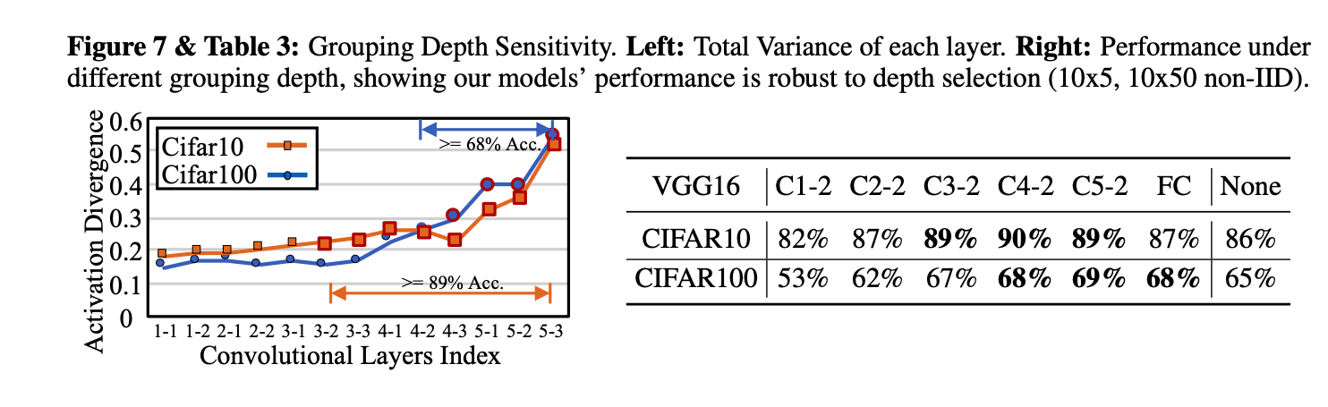
Grouping Depth Analysis.

We also demonstrate that our framework’s performance is robust to the grouping depth hyper-parameter selection in Figure 7. Specifically, our model shows nearly optimal performance 89%⇠90% in large ranges of depth selection, e.g., from C3-2 to C5-2 on CIFAR10. Also, the total variance of the model (a pre-trained model with minimum 50 epoch pre-training) offers good indication of the layer-wise feature divergence.